NGC7635, 04-08 September 2026
One Sky, Four Scopes
In July 2026, I circulated a slide pack proposing a second Seestar collaboration (details of the first collaboration are below). I was hoping for eight telescopes. By the time we had a clear night I had four, which I am told is the normal ratio for anything involving volunteers and the British weather!
Four of us imaged the Bubble Nebula, NGC 7635, on the night of 08 September 2026, from four gardens spread across Suffolk and north Essex. Folding in a session of my own from four nights earlier, we finished with 8.41 hours of usable data on a single object.
That number is worth pausing on, because one telescope could not have produced it. On 8 September from Woodbridge the sky is properly dark — the Sun more than 18° down — for about six hours and forty-five minutes. Our total is longer than the night. And for scale within our own society, the best Seestar image of the Bubble in the OASI archive runs to forty minutes — Paul Whiting’s, as it happens, and the picture I used to advertise the project in the first place.
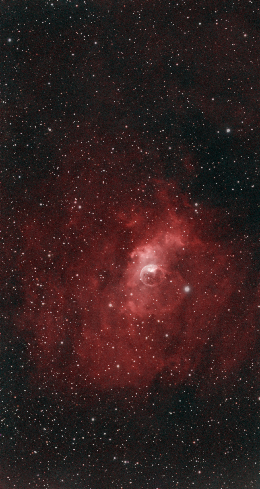
NGC 7635, the Bubble Nebula. 1,064 frames, 8.41 hours, four Seestar S50s, four gardens.
The observers:
- Steve McElvanney, Melton, near Woodbridge,
- Paul Whiting, Felixstowe,
- Andrew Scott, Wivenhoe, near Colchester,
- Steve Tetlow, near Hadleigh.
Each observer used a ZWO Seestar S50 on an equatorial wedge, with the internal dual-band filter. The least and greatest separation of any pair was respectively 15 and 36 kilometres. The telescopes are shown below.
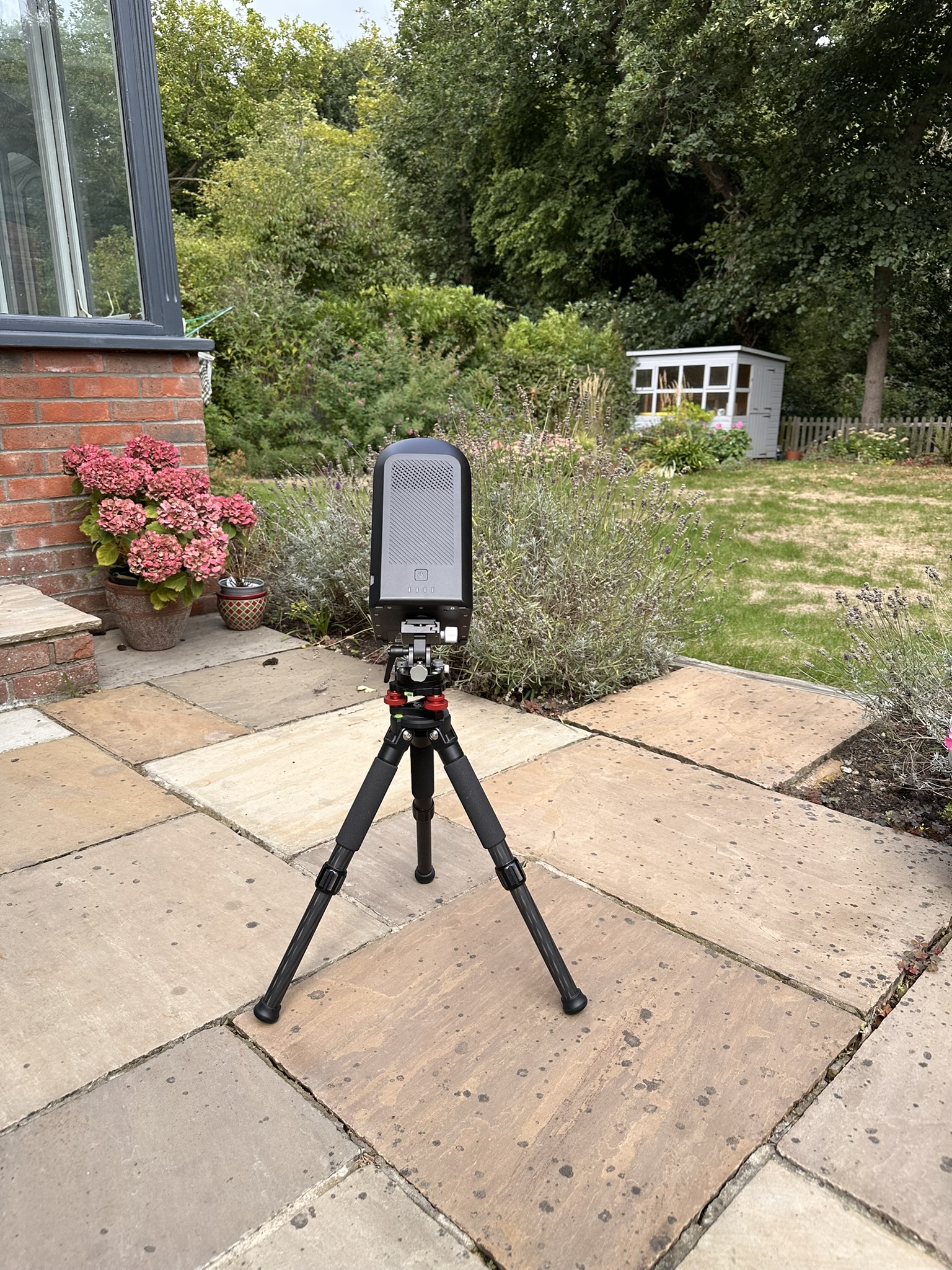
Steve M
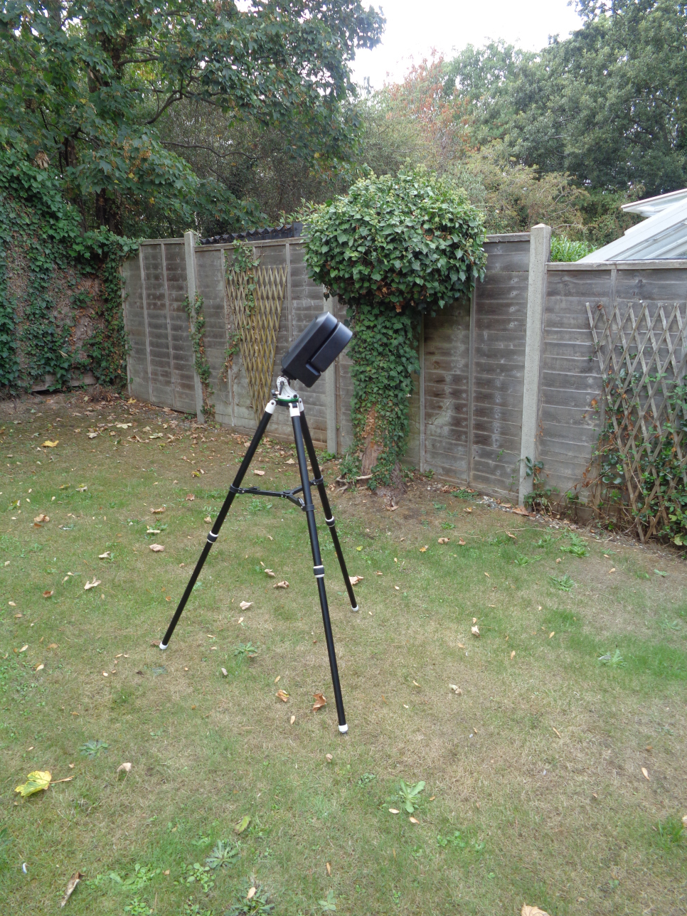
Paul
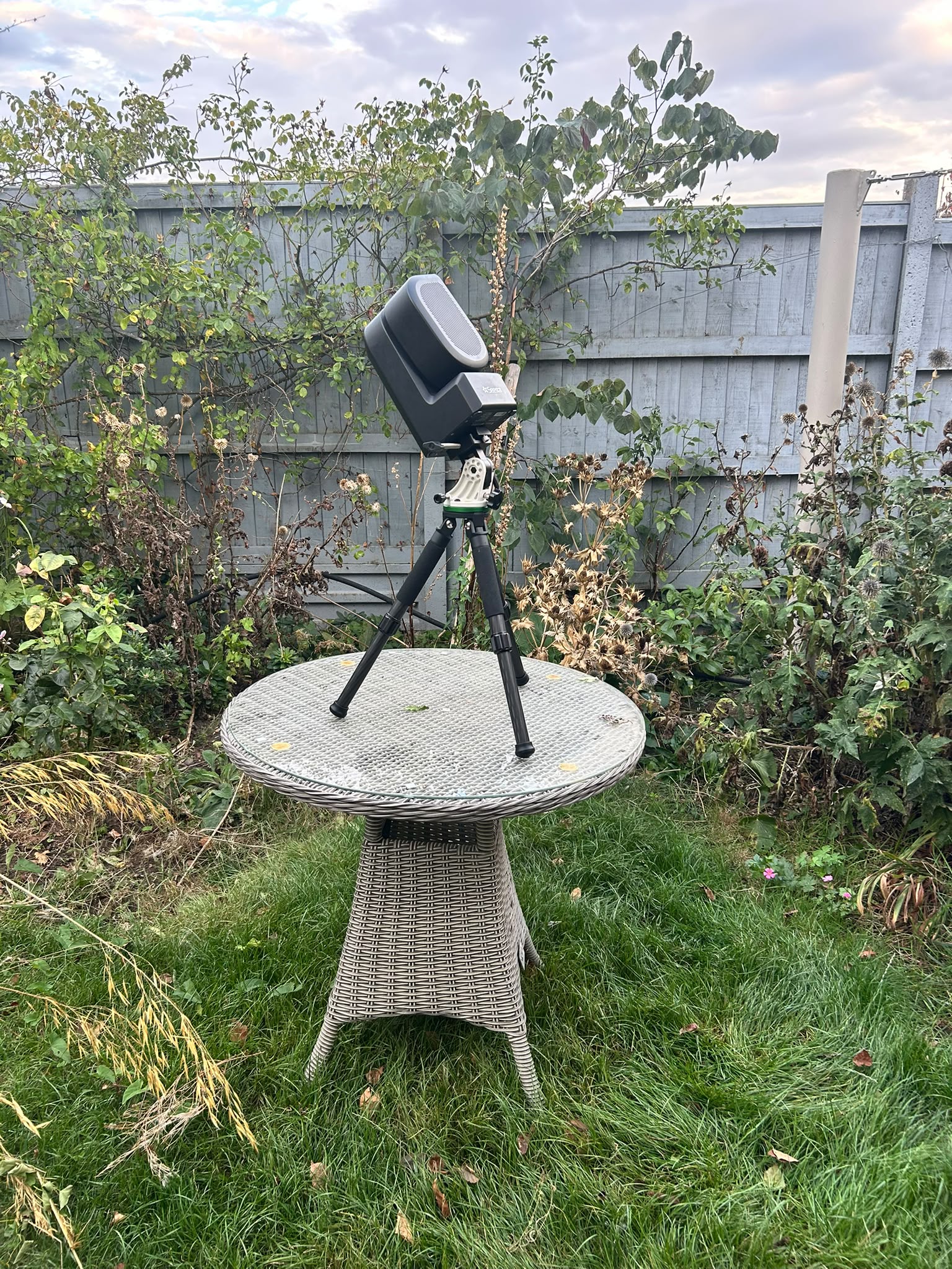
Andrew
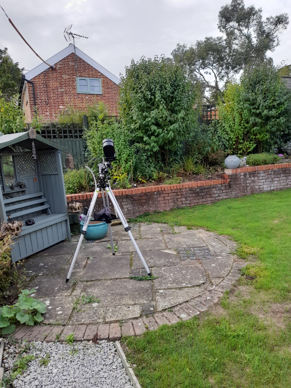
Steve T
The whole method depends upon the filter. It passes only two narrow windows of the spectrum: twenty nanometres around 656 nm, where hydrogen glows red, and thirty nanometres around 501 nm, where doubly ionised oxygen glows blue-green. Everything else — streetlights, moonlight, the general glow of a Suffolk sky — is blocked. An emission nebula like the Bubble radiates almost entirely in those two lines, so the filter discards very little of the target and a great deal of the pollution, which is what makes this kind of imaging possible from an ordinary back garden at all. It also means the finished picture is built from two colours rather than three: the red channel carries hydrogen, and the green and blue channels both carry oxygen.
All processing after capture was done in PixInsight, together with three commercial add-ons from Russell Croman Astrophotography that do specific jobs within it: BlurXTerminator for deconvolution, StarXTerminator to separate the stars from the nebula so the two can be processed independently, and NoiseXTerminator for noise reduction. None of them is free and none is a substitute for integration time, but they have become close to standard equipment.
We did a similar jopint observation once before. In April 2025, Andy Gibbs, Neil Morley, Paul Whiting and I imaged NGC 2403 in Camelopardalis with the same kind of telescope, and that first attempt is worth comparing with the latest one:
The latest collaboration has nearly four times the integration of the earlier one. Two other things changed. The Seestars now support EQ mode on a wedge, which removes field rotation and allows exposures of 30 seconds instead of 10. And we discarded far fewer frames — more on that below, because it was the mistake I most wanted to avoid repeating.
Why collaborate and pool data?
The arithmetic is simple. Noise in a stacked image falls as the square root of the total exposure time. Four hours is twice as good as one; nine hours is three times as good. There is no clever processing that substitutes for it, and on a faint object like the Bubble’s outer shell the difference between two hours and eight is the difference between a smudge and a structure. (The appendix sets out where that square root comes from.)
There is also something the arithmetic does not predict. In every Seestar frame the star images come out slightly elongated, and each unit elongates them in a slightly different direction. When four telescopes’ worth of data is averaged, those directions partly cancel, and the stars in the combined image come out rounder than in any individual contributor’s. The measuring software fits an ellipse to the profile of each star, and the final master’s fitted ellipses have an average eccentricity of 0.575 — which is a way of saying the typical star image is 22 per cent longer than it is wide. The five datasets that went into it ran from 25 to 52 per cent. I had not expected the combination to beat all of them, and it is a genuine argument for collaboration beyond simply piling up hours.
What we had to sort out
Four identical telescopes ought to produce four interchangeable datasets. They do not, and finding out why took rather longer than the imaging.
They are not the same focal length. Every Seestar reports a focal length of 250 mm in its file headers. Plate-solving one frame from each unit gave 251.82, 251.90, 252.20 and 252.20 mm. It is only a 0.15% spread and it changes nothing you can see, but the number in the header is wrong for all of them — and it is not just our four. Other owners’ Seestar images posted online solve to 2.38 arcseconds per pixel, which is what our measured focal lengths give and not what the nominal 250 mm would.
They do not know where they are pointing. Each telescope records the sky coordinates it believes it is looking at. Comparing those against the real position from a plate solve, all four were out by between ten and fourteen arcminutes — roughly a third of the frame’s short dimension. The framing was fine; it was the telescope’s opinion of the framing that was wrong. The practical consequence is that our four fields do not quite coincide: the solved centres are spread over 5.9 arcminutes, and the region covered by all four is about 12% smaller than the best single contributor’s frame.
I had assumed this was our fault and that asking everyone to frame more carefully would fix it. It would not. We all did the same thing — searched for the object in the app and pressed go-to — and the telescopes landed in slightly different places. There is no more careful version of pressing go-to. The 12% is the price of the platform, not a lapse in method.
The sites are not equally good. Paul’s garden in Felixstowe is measurably the brightest and least transparent of the four — about 12% more sky background and 46% more noise per frame than mine at Melton. That is down to geography, and the software handles it: each frame is weighted by its own quality — by a measure built from the star shapes, which penalises a smeared frame as well as a noisy one — so Paul’s contribute proportionally rather than equally. Everybody’s data helps; some of it helps more.
We discarded 86 frames out of 1,154. In 2025, we discarded nearly half, on judgement, and I have since measured what that cost. My own session on 04 September was the first time I did this, and I cut it from 192 frames to 131 by eye. Measuring all 192 afterwards showed the trade was a poor one: the star sharpness improved by 10% and the noise got 21% worse. That is the wrong side of the bargain for a faint target. This time the rule was arithmetic rather than taste — reject a frame if its star sharpness falls far outside the night’s normal spread, or if the number of stars detected drops below 70% of the night’s median, which is what a passing cloud looks like. Under that rule we kept 92%.
Steve Tetlow lost the most — 49 frames, mostly in a bad patch around midnight where his star counts halved while the sky brightness stayed flat, which is thin cloud rather than moonlight. He was asleep at the time, as one should be when the telescope is doing the work, so we will never know for certain. His remaining 303 frames made the best single dataset in the project: lowest noise, most stars detected and the roundest stars of the five, all at once.
Three colours, one nebula
Those 131 frames are worth returning to, because they produced the oddest result of the project. I processed them twice. The first version, which I posted to the OASI WhatsApp group on 05 September, came out violet. Reprocessed, the very same frames came out teal. The combined 1,064-frame master came out red. The images show the effect of different processing:
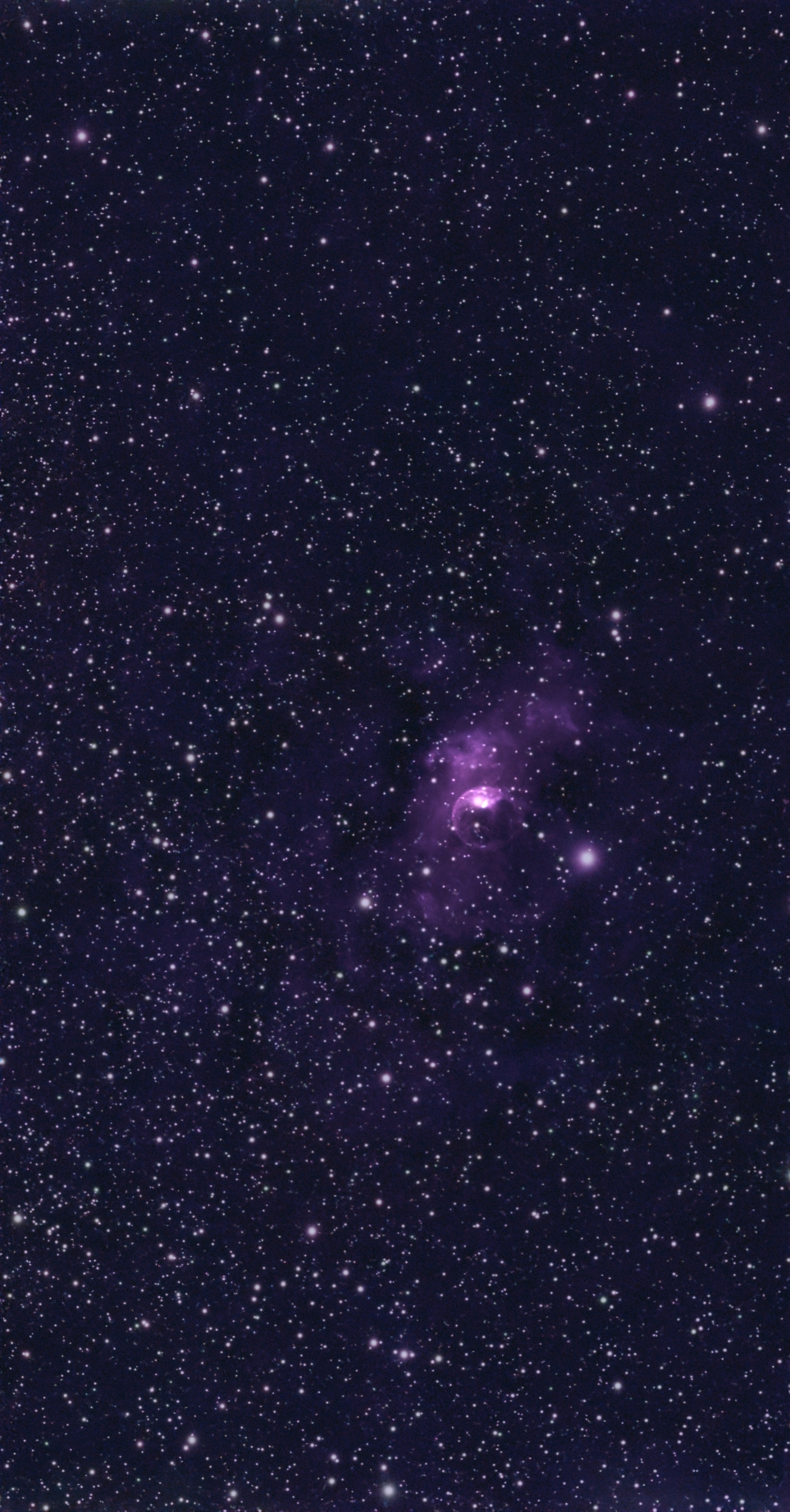
04 Sep, 131 frames: first attempt.
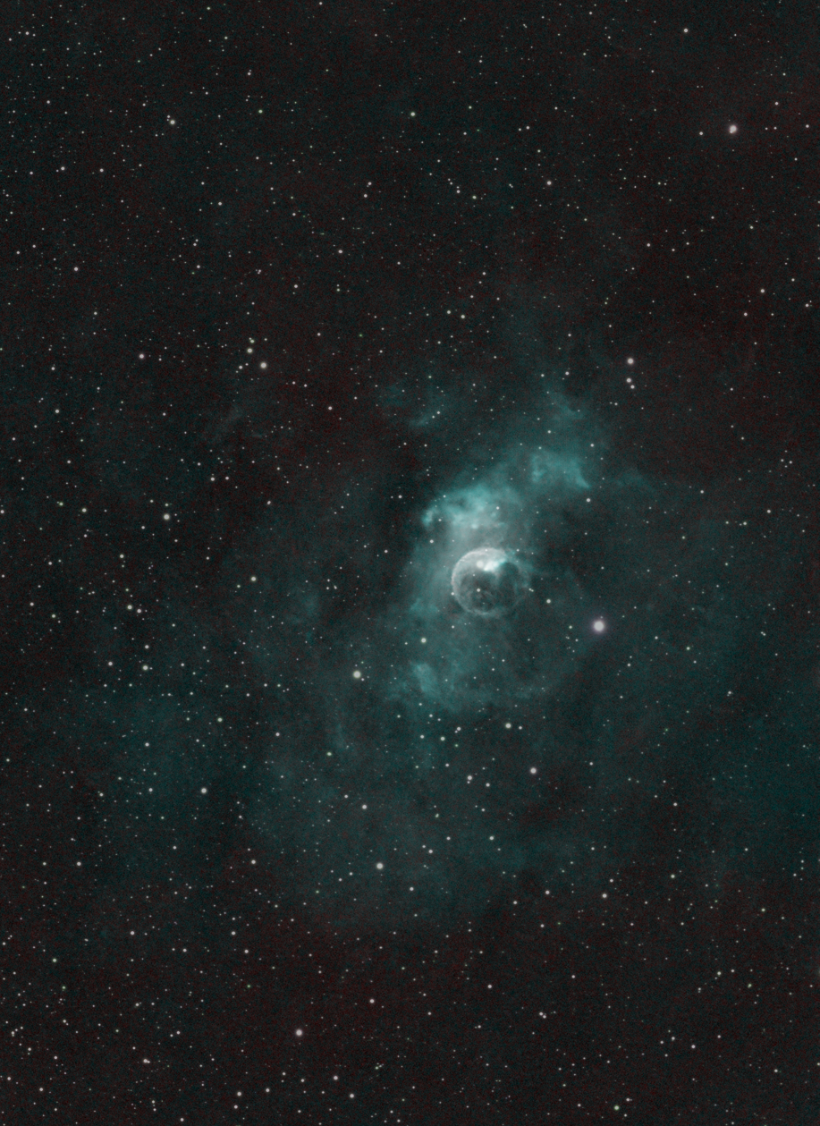
04 Sep, 131 frames: reprocessed.
All five datasets, 1,064 frames.
All three are honest attempts at the same data. What separates them is a single step: colour calibration.
That step deserves explaining, because on the face of it there is no reason it should change the colour of the nebula at all. It never measures the nebula. It calibrates exclusively on stars. The tool is PixInsight’s SpectrophotometricColorCalibration, usually shortened to SPCC, and it works because stellar spectra are known: the European Space Agency’s Gaia satellite has surveyed nearly two billion stars from orbit and published spectra for some 220 million of them, so the colour of almost any star in an amateur frame can simply be looked up. So for any star in the frame you can predict how much light it ought to deliver into each of the three colour channels. Compare that prediction against what the camera actually recorded, across a thousand or so stars, and you have measured the response of the whole chain: filter, sensor and sky together. That response is a property of the equipment and sky rather than the subject of observation, so the three numbers it yields — one multiplier each for red, green and blue — apply to every pixel in the frame. The stars are the standard; the dust in the nebula simply comes along for the ride.
There is a catch, and it is why this went astray. The Seestar’s dual-band filter passes two narrow windows, one at the hydrogen line and one at the oxygen. Stars are continuum sources, radiating across the whole spectrum, so calibrating a pair of narrow bands against broad-spectrum standards is an awkward business at best. SPCC has a narrowband option that has to be ticked deliberately, and on my first attempt I had not ticked it. Left in its default broadband mode the tool assumes the camera saw the whole spectrum through ordinary red, green and blue filters rather than two narrow slices of it, and calibrates accordingly. That produced the violet. For the second attempt on the same 131 frames, and for the final master, the box was ticked and the two wavelengths and bandwidths typed in by hand. Run correctly on the 131 frames, it concluded that red and blue should each come down by about a quarter relative to green — which leaves green dominant, and green is one of the two channels carrying the oxygen signal. That is the teal. Run on the 1,064-frame master, the same step concluded that red should come down by two per cent and blue rise by one, which is barely a correction at all. That is the red. The first two pictures are made from identical frames, and the calibration is the largest difference between them — though not quite the only one. Setting the black point at the end also works on each channel separately, because the sky has to finish neutral, and on the deep master that step subtracted rather more from green and blue than from red, which made the nebula about a third redder again. Both operations are doing legitimate arithmetic on measured quantities. Neither is anybody’s opinion about what colour a nebula ought to be.
The deep version is the one I trust, for a specific reason rather than taste. The calibration works by fitting a line through the measured star colours against the catalogue ones. On the 131 frames — the second attempt, with the filter correctly declared — that line came out sloping the wrong way, which is physically impossible and means the fit itself had failed. So the teal was not a mode error like the violet; it was a correctly configured run on a dataset too shallow to fit. On the 1,064-frame master the same line is clean and positive across 1,282 stars. A correction read off a broken fit is not a calibration.
The star shapes
Every frame captured has slightly elongated stars, and this turned out to be the most interesting thing we found.
The shape a star takes in an image has a name: the point spread function, or PSF. A star is effectively a point of light. Even the largest stars subtend only a few thousandths of an arcsecond as seen from Earth — hundreds of times finer than anything a telescope on the ground can separate, whatever its size — so no image of a star is a picture of the star. Whatever shape it ends up as is a direct measurement of everything that spread the light on its way to the sensor. That makes stars uniquely useful. They are the only objects in the frame whose true appearance is already known, so they become the yardstick for everything else, and the term PSF turns up all over astrophotography software for that reason. Two numbers describe the PSF between them: the full width at half maximum, or FWHM, which is simply how wide the blob is measured halfway up and is the figure usually quoted as the seeing; and the eccentricity, which says how far from circular it is.
Spreading comes in two kinds, and they can be told apart. The atmosphere spreads a star symmetrically, so the blob stays circular. The mount and the optics drag it in one direction, which stretches that circle into an ellipse — and an ellipse is what the fitting software measures. So the short axis of the fitted ellipse tells you what the symmetric blurring alone would have produced, and the amount by which the long axis exceeds it is what the instrument added. Doing that on all five datasets gives, in arcseconds:
The column titled Symmetric blur is mostly the atmosphere, though not purely — a 50 mm aperture cannot make a star sharper than about 2.3 arcseconds however still the air is, and any focus error lands in the same column. The seeing on my own two nights differed by 14%, but my telescope’s contribution moved by only 4%. Something that stays put while the atmosphere changes around it is the instrument, not the sky. And all four instruments show it, at between 5.5 and 6.6 arcseconds.
The three of us imaging at 30 seconds on the same night also measured almost exactly the same blur — 6.44, 6.46 and 6.39 arcseconds — despite being up to 29 km apart. That agreement is worth noticing: the turbulence that limits us is high in the atmosphere and shared across the whole region, not something local to anyone’s garden.
Where does the elongation come from? Partly from the mount. If the telescope does not hold the star perfectly still on the sensor, the star draws a short line during the exposure instead of a point, and a longer exposure draws a longer line. On 04 September I happened to take four frames at 20 seconds before switching to 30, ten minutes apart under identical conditions, and the smear scaled almost exactly with exposure time. That implies a steady drift of about 0.23 arcseconds per second (fourteen arcseconds a minute), enough to draw a seven-arcsecond line in a thirty-second frame, which is what we measure.
But not entirely, because part of it is in the optics. Measuring the same stars separately in the red and green channels shows the red is stretched 24% more than the green. Nothing mechanical can be wavelength-dependent — if the mount drags a star across the sensor, red and green photons take the identical path. So some of what we are seeing is the telescope’s glass, not its motor.
The useful part for anyone else with an S50: this is a known problem and there is a candidate fix. Owners on the Cloudy Nights forum have traced erratic tracking in EQ mode to insufficient friction between the S50’s small round base and the smooth dovetail supplied with the wedge — the base creeps instead of tracking. One reported cross-hatching the mating surface with a scribe and having no further trouble. It is worth ten minutes with a screwdriver before blaming your polar alignment.
There is a happier postscript, and it is worth spelling out for anyone weighing up a Seestar as a first telescope. Much of the blurring can be undone afterwards, by a technique called deconvolution. Because the point spread function can be measured directly from the stars, software can work backwards from it and estimate what the frame would have looked like before the light was spread. This is not sharpening in the photo-editing sense, which simply exaggerates edges and invents nothing; deconvolution is an attempt to reconstruct what was actually there. BlurXTerminator, mentioned earlier, measures the PSF from the image itself and deconvolves each colour channel separately.
It handles our case unusually well, because a smear pointing the same way everywhere in the frame is the easiest thing such software ever has to undo. Across that one step the symmetric blur in the combined master fell by 45%, but the instrumental smear fell by 66%, from 4.13 arcseconds to 1.42. The finished picture has rounder stars than a 10-second alt-az frame would have given us in the first place. It is worth being clear that none of this is a substitute for the hours: deconvolution recovers detail that is present but smeared, and there has to be enough signal there for it to find.
And there is a certain irony in the whole business. The optics have not changed at all; what changed is that a firmware update allowed the Seestar to be polar-aligned on a wedge, which removed field rotation and made 30-second exposures possible. At 10 seconds the smear is around two arcseconds against five or six of blur and you would never see it. Tripling the exposure tripled the smear, and that is the only reason we found it. The problem became visible because the telescopes gained a capability, not because they got worse.
What I would do differently
Agree an exposure length — and expect some units not to hold it. My original brief set 20 seconds as the group standard, and I later asked everyone to use 30 if they could. Andrew’s Seestar would not: its own quality check kept rejecting the longer frames, so it fell back to 20. That is consistent with what we measured, because his unit carries the largest instrumental smear of the four. A group standard is only meaningful if every telescope can actually meet it, so ask people to report what they ended up using.
Accept that the fields will not match. I considered asking everyone to use the Seestar’s mosaic mode so each unit covered a deliberately wider area, which would make the common region much larger. But a mosaic needs something like four times the integration to reach the same depth, and on a faint target depth is the entire point. Better to lose the 12% and keep the hours.
Don’t fix a date. We planned for 12 September. Clear Outside showed one clear Tuesday and cloud for the rest of the week, so we moved everyone to the 08 September at a day’s notice, and that is why the project happened at all. Capture when you can and let the processing sort it out afterwards.
Measure before rejecting. The temptation to keep only the pretty frames is strong and it is usually wrong.
The numbers
Comparing my single-telescope session on 04 September with the collaborative effort:
The square-root rule predicts an improvement of 2.35× due to the extra exposure. We achieved 2.51×, which is better than it should be — not because the arithmetic is wrong, but because the dataset that took us from five and a half hours to eight and a half happened to be the best of the five rather than a typical one. The more interesting comparison is against the best single contributor, because it shows what the collaboration bought beyond sheer volume:
Deeper, more stars, rounder stars — and a field 12% smaller. The rounder stars are the part no amount of time on one telescope would have achieved.
For a sense of how far this can go, a group calling itself the Seestar Collective has done the same thing on the same object with about thirty contributors and 270 hours. We are four people and 8.41 hours, which is a long way behind — but it is the same method, and it evidently keeps working as you add people.
We will do this again. There is still room for another four telescopes.
Appendix — where the square root comes from
Two quantities matter. The signal S is the light from the object landing in a given pixel during one exposure. The noise σ is the random fluctuation about that value from one exposure to the next.
Stack N frames. The signal adds up in step, because every frame records the same object in the same place, so the total is N × S. The noise does not, because it is random and independent from one frame to the next — and independent random quantities add in quadrature, meaning their variances add rather than their standard deviations. For N frames each carrying noise σ:
σtotal = √(σ2 + σ2 + ... + σ2) = √N·σ .
Divide one by the other and the signal to noise ratio (SNR) after N frames is
SNRN = N·S / (√N·σ) = √N·(S/σ) ,
which is the square-root law. A hundred frames carry a hundred times the signal but only ten times the noise, so the result is ten times cleaner than a single frame. It also explains why the returns diminish so brutally: to double the quality you must quadruple the frames. The following graph shows how signal and noise grow with the number of frames stacked; the gap between the two lines is the whole point of the exercise.
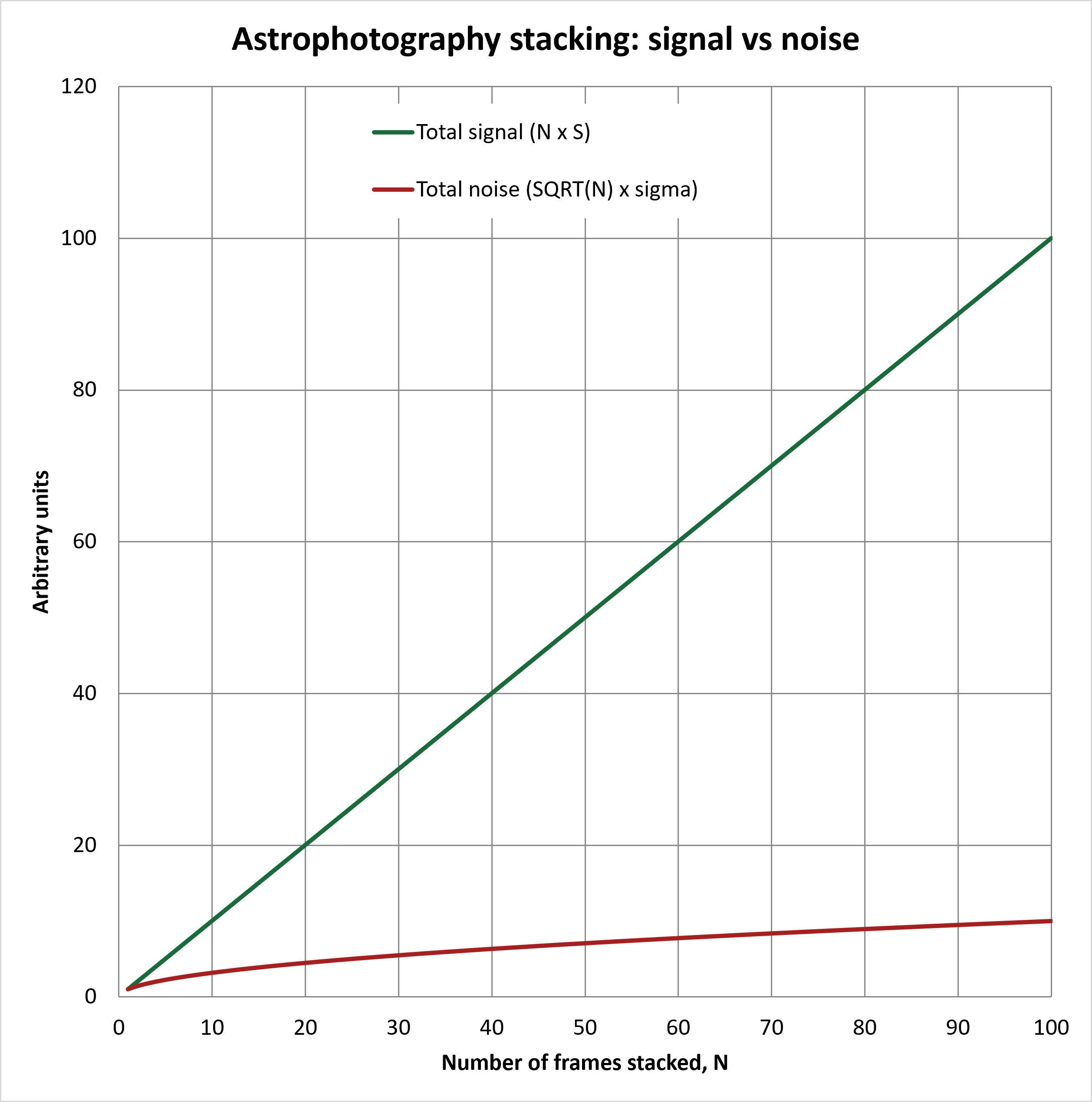
Signal and noise against the number of frames stacked.
Where the noise comes from is worth a sentence, because it sets a floor nothing can get under. Light is grainy: photons arrive at random, according to a Poisson process. The latter has a standard deviation equal to the square root of its mean. A pixel that collects 10,000 photons therefore carries about 100 photons of noise whether you like it or not, and no processing removes it — it can only be outgrown by collecting more. On top of that sits read noise, added by the camera electronics each time the sensor is read out, and that one is charged per frame rather than per second. Three hundred ten-second frames and a hundred thirty-second frames hold the same fifty minutes of light, but the first pays the read-noise toll three times as often. That is the quiet argument for longer subs, and the second reason EQ mode mattered.
So much for theory. What we measured was this. Going from 761 frames to the full 1,064 took the integration from 5.85 hours to 8.41, and the square-root law predicts the noise should improve by √(8.41 ∕ 5.85) = 1.199. It improved by 1.255 — slightly better than the law allows, because the dataset we added was the best of the five rather than an average one, so it was not simply more of the same.
Across the whole project we fall short of the ideal, as everyone does. A single sub measures a noise of 2.19×10⁻⁴ and the finished 1,064-frame master 1.430×10⁻⁵, an improvement of 15.3 times where a perfect √1064 would give 32.6. Just under half. The missing half goes mostly on registration: every frame has to be resampled onto a common pixel grid before it can be added, and interpolation correlates neighbouring pixels — which is precisely what the arithmetic above assumes does not happen. Normalisation and weighting take a further share. Budgeting on roughly half the theoretical figure is about right, and it is another reason to prefer real extra hours over clever processing.
Steve McElvanney, with assistance from Anthropic's Claude.